
Tree in Design and Analysis of Algorithm Study Notes with Examples
Tree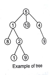
A tree is the data structure that are based on hierarchical tree structure with set of nodes. It is a acyclic connected graph with one or more children nodes and at most one root node.
In a tree, there are two types of node
- Internal nodes All nodes those have children nodes are called as internal nodes.
- Leaf nodes Those nodes, which have no child, are called leaf nodes.
Tree terminology
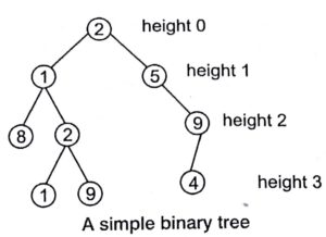
The depth of a node is the number of edges from the root to the node. The height of a node is the number of edges from the node to the deepest leaf. The height of a tree is the height of the root.
Binary Tree
A binary tree is a tree like structure that is rooted and in which each node has at most two children and each child of a node is designated as its or right child.
Types of Binary Trees
The types of binary trees depending on the trees structure are as given below
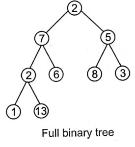
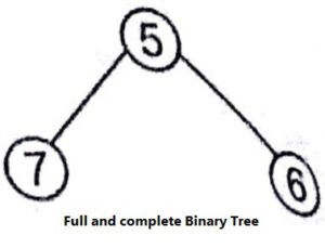
Full Binary Tree
A full binary tree is a tree in which every node other than the leaves has two children or every node in a full binary tree has exactly 0 or 2 children.
Complete Binary Tree
A complete binary tree is a tree in which every level, except possibly the last, is completely filled.
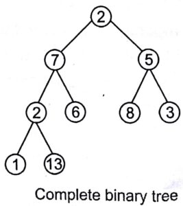
The number n of nodes in a binary tree of height h is at-least n = h + 1 and atmost
N=21” – 1, where h is the depth of the tree.
Tree Traversal
There are three standard ways of traversing a binary tree T with root R..
These three ways are given below
Preorder
- Process the root R.
- Traverse the left subtree of R in preorder.
- Traverse the right subtree of R in preorder.
Inorder
- Traverse the left subtree of R in inorder.
- Process the root R.
- Traverse the right subtree of R in inorder.
Postorder
- Traverse the left subtree of R in postorder.
- Traverse the right subtree of R in postorder.
- Process the root R.
Breadth First Traversal (BFT)
The breadth first traversal of a tree visits the nodes in the order of them depth in the tree. Breadth first traversal first visits all the nodes at depth zero (i.e., root), then all the nodes at depth one and so on.
Depth First Traversal (DFT)
Depth first traversal is an algorithm for traversing or searching a tree, tree structure or graph. One starts at the root and explores as far as possible along each branch before backtracking.
Key Points
- Queue data structure is used for this traversal.
- Stack data structure is used for traversal
Binary Search Tree
A binary search tree is a binary tree, which may also be called an ordered or sorted binary tree.
A binary search tree has the following properties.
- The left subtree of a node contains only nodes with keys less than the node’s key.
- The right subtree of a node contains only nodes with keys greater than the node’s key.
- Both the left subtrees and right subtrees must also be binary search trees.
Pseudo Code for Binary Search Tree (BST)
The pseudo code for BST is same as binary tree because it also has node with data, pointer to left child and a pointer to right child.
struct node;
int data;
struct node * left;
struct node * right;
{
// A function that allocates a new node with the given data and NULL // left and right pointers struct node* newNode (int data)
}
struct node* newNode = (struct node*) malloc (sizeof (struct node));
newNode —> data = data;
newNode —> left = NULL;
newNode —> right = NULL;
return (newNode) ;
Insert a Node into BST
/* Given a binary search tree and a number, inserts a new node with the given number in the correct place in the tree*/
struct node * insert (struct node* node, int data).
/* If the tree is empty, return a new, single node */
if (node ==NULL)
return (newNode (data));
else
{
/* Otherwise, insert a newnode at the appropriate place, maintaining the property
of BST */
if (data < node —> data )
node —> left = insert (node —> left , data) ;
else
node —> right =insert (node—> right, data) ;
return node ;
}
}
In a BST, insertion is always at the leaf level, traverse the BST, comparing the new value to existing ones, until you find the right point, then add anew leaf node holding that value.
Deletion From a Binary Search. Tree
Deletion is the most complex operation on a BST, because the algorithm must result in a BST. The question is “what value should replace the one deleted?”
Basically, to remove an element, we have to follow two steps
- Search for a node to remove.
- If the node is found, run remove algorithm..
Procedure for Deletion of a Node From BST
There are three cases to consider
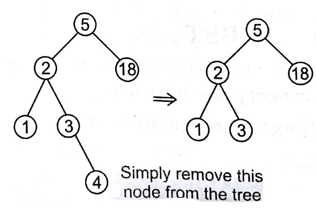
Deleting a Leaf Node (Node with No Children)
Deleting a leaf node is easy, as we can simply remove it from the tree.
Remove 4 from a BST given below
Deleting a Node with One Child
Remove the node and replace it with its child.
Remove 18 from a BST given below
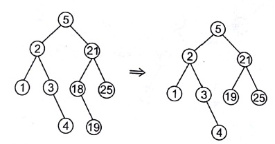
- In this case, node is cut from the tree and node’s subtree directly links to the parent of the removed node
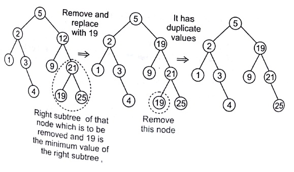
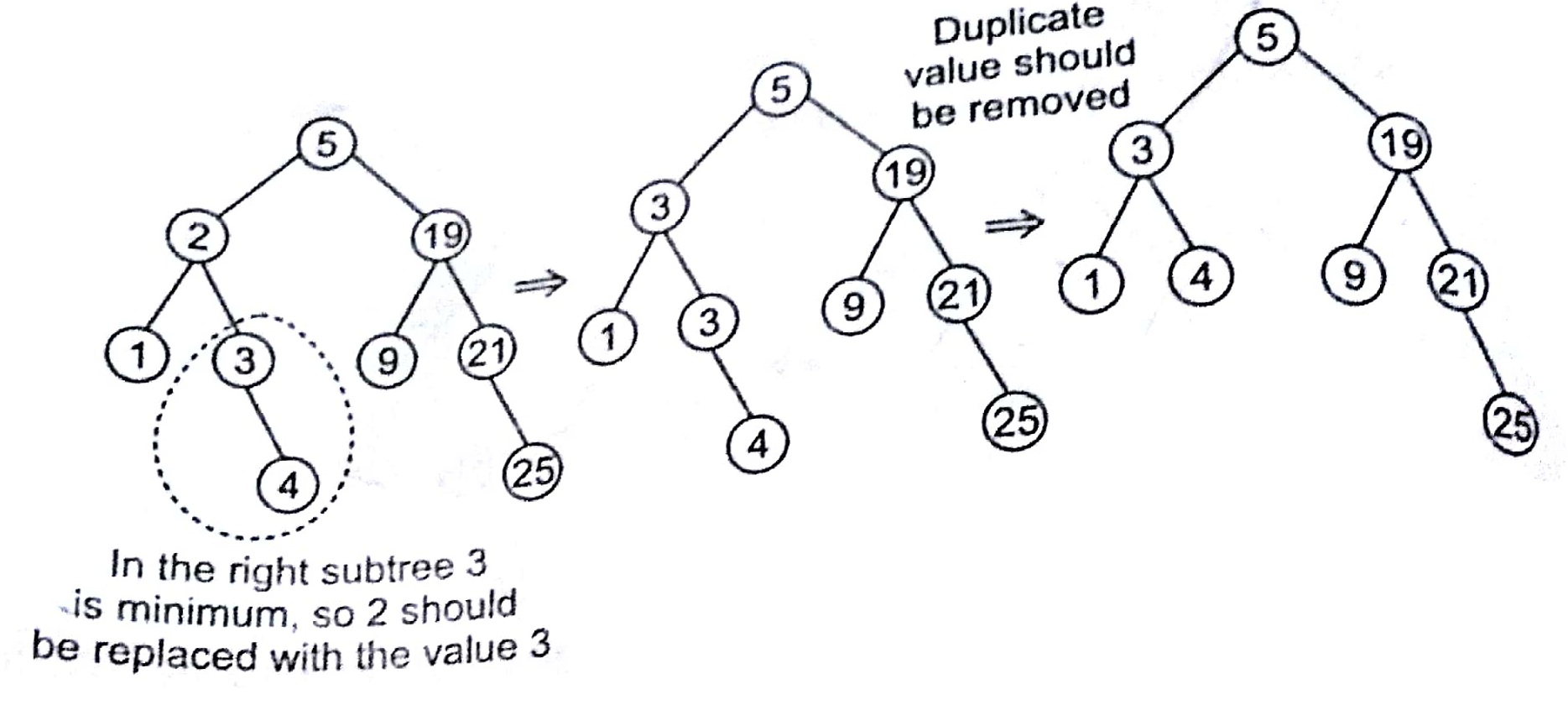
Deleting a Node with Two Children
This is the most complex case to solve it, we use the approach as given below
- Find a minimum value in the right subtree.
- Replace value of the node to be removed with found minimum. Now, right subtree contains a duplicate.
- Apply remove to the right subtree to remove a duplicate.
e.g., Remove 12 from the given BST
Now If, we delete 2 from this BST, then
Implementation of BST Deletion
void deleteNode (struct node * treePtr, int value)
{
struct node rightPtr, leftPtr;
struct node current =*treePtr, * parentPtr, *temp;
if (! current)
{
printf (“The tree is empty or has not this node”);
return;
}
if (current →data == value)
{
/* It’s a leaf node */
if ( ! current —> rightPtr && ! current →leftPtr)
{
* treePtr = NULL;
free (current);
}
/* the right child is NULL and left child
is not null t *1
else if (! current → rightPtr)
{
* treePtr = current → leftPtr ;
free (current);
/* the node has both children */
else
}
temp = current —> rightPtr ;
/* the rightPtr with left child */
if ( ! temp —>leftPtr)
temp —> leftPtr = current —> leftPtr;
. /* the rightptr have left child */
else
{
/* find the smallest node in right subtree */
while (temp →leftPtr )
{
/* record the parent node of temp */
parentPtr = temp;
temp = temp —* leftPtr;
}
parentPtr →leftPtr = temp —> rightPtr ;
temp → leftPtr = current → leftPtr
temp —> rightPtr = current —> rightPtr;
}
* treePtr = temp;
tree (current);
}
else if (value → current —> data )
{
/* search the
deleteNode (& ( current →rightPtr),value);
}
else if (value < current data)
{
deleteNode (& (current→rightptr)
value);
}
}
Average Case Performance of Binary
Search Tree Operations
Internal Path Length (IPL) of a binary tree is the sum of the depths of its nodes. So, the average internal path length T(n) of binary search trees with n nodes is 0(n log n).
The average complexity to find or insert operations is T(n) = 0 (log n).
Improving the Efficiency of Binary Search Trees
- Keeping the tree balanced.
- Reducing the time for key comparison.
Balanced Trees
Balancing ensures that the internal path lengths are close to the optimal n log n. A balanced tree will have the lowest possible overall height.
There are many balanced trees
- AVL Trees 2. B-Trees
AVL Trees
An AVL (Adelson-Velskii and Land is) is a binary tree with the following additional balance property.
- For any node in the tree, the height of the left and right subtrees can differ by atmost.
- The height of an empty subtree is —1.
The method to keep the tree balanced is called node rotation. AVL trees are binary trees those use node rotation upon inserting a new node.
An AVL is a binary search tree which has the following properties
- The subtrees of every node differ in height by atmost one.
- Every subtree is an AVL tree.
Every node of an AVL tree is associated with a balance factor. Balance factor of a node = Height of left subtree — Height of right subtree A node with balance factor — 1, 0 or 1 is considered as balanced.
An AVL tree is shown here.

This AVL tree is balanced and a BST.

It is a BST but not AVL tree because it is not balanced. At node 10, the tree is unbalanced. So, we have to rotate this tree.
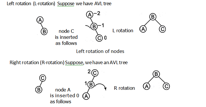
Rotations
A tree rotation is required when we have inserted or deleted a rode which leaves the tree in an unbalanced form.
There are four types of rotations as given below

Greedy Algorithms
Greedy algorithms am simple and straight forward, They are short sighted in their approach in the sense that they take decisions on the basis of information at I land will worrying about the effect of this decisions in the future. They are as follows
- Easy to implement.
- Easy lo invent and require minimal amount of resources.
- Quite efficient.
Note: Greedy approaches are used to solve optimization problems.
Feasibility
A feasible set is promising, if it can be extended to produce not merely as solution, but an optimal solution to the problem. Unlike dynamic programming which solves the sub-problems bottom-up strategy, a Greedy strategy usually progress in a top-down fashion, making one Greedy choice after another, reducing each problem to a smaller one.
Optimization Problems
An optimization problem is one in which you want to find not just a solution, but the best solution. A Greedy algorithm sometimes works well for optimization problems.
Examples of Greedy Algorithms
The examples based on Greedy algorithms are given below
Activity Selection Problem
If there are n activities, S={1,2,… ,n), where S is the set of activities.Activities are to be scheduled to use some resources, where each activity I has its starting time Si and finish time f with Si ≤ fi, i.e., the two activities and j are non-interfering, if their start-finish intervals do not overlap, So,
(Si, f,)∩ (Sj, fj) =Ф
The activities i and j are compatible, if their time periods are disjoint. In this algorithm, the activities are firstly sorted in an increasing order, according to their finish time. With the Greedy strategy, we first select the activity With smallest interval (Fi – Si) and schedule it, then skip all activities, that are not compatible with the current selected activity and repeats this process until all the activities are considered.
Algorithm for Activity Selection Problem
Activity_Selection_Problem (S,f,i , j)
{
A←1
M← i+1
while m < j and Sm < fi
dom←m+1 if m < j
then return A= A U Activity_Selection_Problem (S, f, m, j)
else
return (Ф)
The running time of this algorithm is θ(n) assuming that the activities are already sorted.
Fractional Knapsack Problem
There are n items; ith item is worth vi dollars and weights wi pounds, where vi and weo are integers. Select items to put in Knapsack with total weight < W, so that total value is maximized. In fractional Knapsack problem, fractions of items are allowed.
– Key Points
- To solve the fractional problem, we have to compute the value per weight for each item.
- According to Greedy approach, item with the largest value per weight will be taken first.
- This process will go on until we can’t carry any more.
Algorithm of Fractional Knapsack
Greedy_Fractional_Knapsack (G, n, W)
{
/* G is already sorted by the value per weight of items order *1
Rw = W, i = 1
while ( (Rw > 0) and (i≤n)) do
if (Rw > wi) then fi = 1
else f; = Rey/w;
Rw = Rw, — fi * Wi
i+ +
end while return F
}
where F is the filling pattern i.e., F ={ fi, f2,……fn} and 0≤fi, ≤ 1 denotes, the fraction of the ith item.
Analysis
If the items are already sorted into the decreasing order of value per weight, then the algorithm takes 0(n) times.
Task Scheduling Problem
There is a set of n jobs, S = { 1, 2, … n}, each job i has a deadline di 0 and a profit pi 0. We need one unit of time to process each job. We can earn the profit pi, if job i is completed by its deadline. To solve the problem of task scheduling sort the profit of jobs (pi) into non-decreasing order.
After sorting, we will take the array and maximum deadline will be the size of array. Add the job i into the array, if job i can be completed by its deadline. Assign i to the array slot of [r — 1, r], where r is the largest such that 1 < r1. This process will be repeated, until all jobs are examined.
Note: The time complexity of task scheduling algorithm is 0(n2).
Minimum Spanning Tree Problem
Spanning Tree: A spanning tree of a graph is any tree that includes every vertex in the graph. More formally, a spanning tree of a graph G is a sub-graph of G that is a tree and contains all the vertices of G. Any two vertices in a spanning tree are connected by a unique path. The number of spanning trees in the complete graph Kn is nn -2.
Minimum Spanning Tree: A Minimum Spanning Tree (MST) of a weighted graph G is a spanning tree of G whose edges sum is minimum weight.
There are two algorithms to find the minimum spanning tree of an undirected weighted graph.
Kruskal’s Algorithm
Kruskal’s algorithm is a Greedy algorithm. In this algorithm, starts with each vertex being its component. Repeatedly merges two components into on.e by choosing the light edge that connects them, that’s why, this algorithm Is edge based algorithm. According to this algorithm.
(V, E) is a connected, undirected, weighted graph.
Scans the set of edges in increasing order by weight. The edge is selected such that
- Acyclicity should be maintained.
- it should be minimum weight.
- When tree T contains n — 1 edges, also must terminate.
uses a disjoint set of data structure to determine whether an edge connects vertices in different components.
Data structures: Before formalizing the above idea, we must review the disjoint set of data structure.
MAKE_SET (v): Create a new set whose only member is pointed to by v. Note that for this operation, v must already be in a set.
FIND_SET (v): Returns a pointer to the set containing v.
UNION (u, v): Unites the dynamic sets that contain u and v into a new set that is union of these two sets.
Algorithm for Kruskal
Start with an empty set A and select at every stage the shortest edge that has not been chosen or rejected, regardless of where this edge is situated in the graph.
KRUSKAL (V, E, w )
{
A ←ɸ
for each vertex v ϵ V
do MAKE_SET (v)
Sort E into non-decreasing order by weight w
for each (u, v) taken from the sorted list
do if FIND_SET (u) # FIND_SET (v)
then A ←A u {(u, v) }
UNION (u, v)
return A
}
Analysis of Kruskal’s Algorithm
The total time taken by this algorithm to find the minimum spanning tree is 0(Elog2 E) (if edges are already sorted). But the time complexity, if edges are not sorted is 0(Elog2 V).
Prim’s Algorithm
Like Kruskal’s algorithm, Prim .‘s algorithm, is based on a generic minimum spanning tree algorithm. The idea of Prim’s algorithm is to find the short,1 path in a given graph. The Prim’s algorithm m has the property that the edges in the set A always form a single connected tree.
In this, we begin with some vertex v in a given graph G = (V ,E), defining the initial set of vertices A. Then, in each iteration, we choose a minimum weight edge (u, v), connecting a vertex v in the set A to the vertex u outside of set A. Then, vertex u is brought into A. This tree is repeated, until spanning tree is formed.
This algorithm uses priority queue Q.
- Each object is a vertex in V — VA.
- Key of v is minimum weight of any edge (u, v), where u E VA.
- Then, the vertex returned by ,EXTRACT_MIN is v such that there exists u E VA and (u ,v) is a light edge crossing (VA,V — VA).
Algorithm for Prim
PRIM (V, E,w,r)
{
Q ←ɸ
for each uϵ V
do key [u] <–
[u] ←NIL
INSERT (Q , u)
DECREASE_KEY (Q,r,o)
While Q≠ɸ
do u ←EXTRACT_MIN (0)
for each v ϵ Adj [u]
do if v ϵ 0 and w (u, v) < key [v]
then [v] ←u
DECREASE_KEY (0, v, w (u, v) )
}
Analysis of Prim’s Algorithm
The time complexity for Prim’s algorithm is 0 (E log2 V)
Dynamic Programming Algorithms
Dynamic programming approach for the algorithm design solves the problems by combining the solutions to sub-problems, as we do in divide and conquer approach. As compared to divide and conquer, dynamic programming is more powerful.
Dynamic programming is a stage-wise search method suitable for optimization problems whose solutions may be viewed as the result of a sequence of decisions.
Greedy versus Dynamic Programming
For many optimization problems, a solution using dynamic programming can be unnecessarily costly. The Greedy algorithm is simple in which each step chooses the locally best. The drawback of Greedy method is that the computed global solution may not always be optimal.
- Both techniques are optimization techniques and both build solution from a collection of choices of individual elements. Dynamic programming is a powerful technique but it often leads to algorithms with higher running times.
- Greedy method typically leads to simpler and faster algorithms.
- The Greedy method computes its solution by making its choices in a serial forward, never looking back or revising previous choices.
- Dynamic programming computes its solution bottom up by synthesizing them from smaller subsolutions and by trying many possibilities and choices before it arrives the optimal set of choices.
Approaches of Dynamic Programming
The dynamic programming consists of following sections
0-1 Knapsack
The idea is same as fractional knapsack but the items may not be broken into smaller pieces, so we may decide either to take an item or to leave it, but we may not take a fraction of item. Only dynamic programming algorithm exists.
Single Source Shortest Paths
In general, the shortest path problem is determine one or more shortest path between a source vertex and a target vertex, where a set of edges are given. We are given a directed graph G= (V,E) with non-negative edge weight and a distinguished source vertex, s ϵ V. The problem is to determine the distance from the source vertex to every other vertex in the graph.
Dijkstra’s Algorithm
Dijkstra’s algorithm solves the single source shortest path problem on a weighted directed graph. It is Greedy algorithm. Dijkstra’s algorithm starts at the source vertex, it grows a tree T, that spans all vertices reachable from S.
Algorithm for Dijkstra
DIJKSTRA (V, E, W, S)
{
INITIALIZE_SINGLE_SOURCE (V, S)
S←ɸ
Q←V # insert all vertices into E)
while Q≠ɸ
do u←EXTRACT_MIN (0)
S<–S u {u}
for each vertex v ϵ Adj [u]
do RELAX (u, v, w)
}
INITIALIZE_SINGLE_SOURCE (G, S)
{
for each vertex v E V[G]
do d[v] <— ∞
[v] ←NIL
d [S] ←o
}
RELAX(u,v,w)
{
if d[v] > d[u]+ w (u, v)
then d[v] <— d[u]+ w (u, v)
}
[v] ←u
have two sets of vertices
S = Vertices whose final shortest path weights are determined
Q = Priority queue = V— S.
Sorting in Design and Analysis of Algorithm Study Notes with Example
Follow Us on Social Platforms to get Updated : twiter, facebook, Google Plus
Learn Sorting in Handbook Series: Click here