
Sorting in Design and Analysis of Algorithm Study Notes with Example
Sorting
In Computer Science, sorting operation is used to put the elements of list in a certain order, i.e., either in non-decreasing or decreasing order.
Sorting can be of two types
- In-place sorting
- Stable Sorting
In-place Sorting
The in-place sorting algorithm does not use extra storage to sort the elements of a list. An algorithm is called in-place as long as it overwrites its input with its output. Those algorithms, which are not in-place, are out of place algorithms.
Stable Sorting
Stable sorting algorithm maintain the relative order of records with equal values during sorting and after sorting operation or we can say that a stable sorting algorithm is called stable, if it keeps elements with equal keys in the same relative order as they were in the input.
Divide and Conquer Approach
The divide and conquer approach is based on the recursion or it works by recursively breaking down a problem into two or more sub problems, until these becomes simple enough to be solved directly. The solutions of the sub problems are then combined to give a solution to the original problem. ,
Methods of Sorting
There are different sorting techniques as given below
Bubble Sorting
Bubble sorting is a simple sorting algorithm that works by repeatedly stepping through the list to be sorted, comparing each pair of adjacent items and swapping them, if they are in random or unorganized order. This sorting technique go through multiple passes over the array and each pass moves the largest (or smallest) element to the end of the array.
pseudo Code for Bubble Sorting
void Bubble Sort (int a[ ], int n)
{
int i , temp,j;
for (i=1; i <=n; i++)
{
for(j=1; j<=i; j++)
{
if (a[j] > a [j +1])
{
temp= a [j],
a [j]= a [j +1];
a [j +1] = temp;
}
}
}
}
The internal loop is used to compare adjacent elements and swap elements, if they are not in order. After the internal loop has finished the execution, the largest element in the array will be moved at the top. The external loop is used to control the number of passes.
Flow Chart for Bubble Sorting

Analysis of Bubble Sort
Generally, the number of comparisons between elements in bubble short can be stated as follows
(n – 1) + (n – 2) +…+ 2 + 1 = n (n – 1)/2 = 0 (n2)
In any case (worst case, best case or average case) to sort the list in be ascending order, the number of comparisons between elements would b same. But the time complexity is different.
The time complexity of bubble sort in all three cases is given below
- Best case 0 (n) Average case 0 (n2) • Worst case 0 (n2)
Insertion Sorting
The insertion sort only passes through the array once. Therefore, it is very fast and efficient sorting algorithm with small arrays.
Key Points
- This algorithm works the way you might sort a hand of playing cards
- We start with an empty left hand [sorted array] and the cards face down on the table [unsorted array].
- Then, remove .one card [key] at a time from the table [unsorted array] and insert it into the correct position in the left hand [sorted array].
- To find the correct position for the card, we compare it with each of the cards already in the hand, from right to left.
Pseudo Code of Insertion Sort
int insertionsort (int a[], int n)
{
int i , j, key;
for (j =2; j<= n; j -H-)
{
key = a [j];
i =j —1;
while (i > && a [i] > key)
{
a [1 +1] = a [i] ;
i=i – 1;
}
a [i +1] = key;
}
}
Flow Chart for Insertion Sorting

Analysis of Insertion Sort
The running time depends on the input. An already sorted sequence is easier to sort.
The time complexity of insertion sort in all these cases is given below .
Worst case Input is in reverse sorted order
n
. T(n) = E 0(j) =0 (n2)
j=2
Average case All permutations equally likely
T(n) = I 0 (j /2) = 0 (n2) j = 2
Best case If array is already sorted
T(n) = 0(n)
Merge Sort
Merge sort is a comparison based sorting algorithm. Merge sort is a stable short, which means that the implementation preserves the input order of equal elements in the sorted output array.
Merge sort is a divide conquer algorithm The Performance is independent of the initial order of the array items.
Pseudo Code of Merge Sort
void mergeSort (int a [ ], int first, int last)
{
if (first < last)
{
Int mid= (first+ last)/2;
mergeSort (a, first, mid);
mergeSort (a, mid + 1, last);
//Divide the array into pieces
merge (a, first, mid, last);
//Small pieces are merged
}
}
void merge (int a [],
int first, int mid, int last)
{
int c[100]; // temporary array
int i , j, k, m;
i = first ;
j= mid;
k=mid+1; m= first;
while (first < = last)
{
while (i <=j && k <= last)
{
if (a [1] < a [lc])
{
c[m]=a [1];
i ++;
m++;
}
else
{
c[m]= a [k];
m++;
k ++;
}
while(1<=j)
{
c [m] = a [i];
i++;
m ++ ;
}
while (k <= last)
{
c [m] = a [k];
m++;
K++;
}
for (1=0; i < = last; i++)
{
a[i] = c[i];
}
}
}
Key Points
There are three main steps in merge sort algorithm
- Divide An array into halves, until only one piece left.
- Sort Each half portion.
- Merge The sorted halves into one sorted array.
Analysis of Merge Sort
The merge sort algorithm always divides the array into two balanced lists. So, the recurrence relation for merge sort is

The time complexity of merge sort in all three case (best, average and worst) is given below
- Best case 0(n log2 n)
- Average case 0 (n log2 n)
- Worst case 0 (n loge n)
Quick Sort
It is in-place sorting, since it uses only a small auxiliary stack. It is also known as partition exchange sort. Quick sort first divides a large list int smaller subsists. Quick sort can then recursively sort the subsists.
key Points
- It is a divide and conquer algorithm.
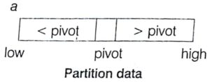
- In quick sort algorithm, pivot element is selected and arrange all the items in the lower part are less than the pivot and all those in the upper part greater than it.
The pseudo code of quick sort
int quicksort (int a [ J, int low, int high)
{
int pivot;
if (low < high)
{
pivot =partition (a, low, high); quicksort (a, low, pivot —1); quicksort (a, pivot +1,high);
}
}
int partition (int a [ J, int low, int high)
{
int temp;
int i = low;
int p= low;
int q = last; while (i < j)
{
while (a [p] < = a [1] && i< last)
{
I++;
}
while (a[q] > a [i])
{
j – -;
}
if (p<q)
{
temp= a [p];
a[p]= a[q];
a [q]= temp;
}
temp = a [i];
a [i]= a [q];
a [q] = temp;
return q;
}
Analysis of Quick Sort
The time complexity calculation of quick sort in all three cases is given below
Worst case: 0(n2) This happens when the pivot is the smallest
(or the largest) element. Then, one of the partitions is empty and we repeat recursively the procedure of n –1 elements.
The recurrence relation for worst case
T(n) = T(n – 1) + cn, n > 1
T(n)=T(n – 2) + c(n – 1) + cn
T(n)=T(n – 3) + c(n 2)+c(n-1)+cn
Repeat upto K – 1 times, we get
T(n) = T(1) + c(2 + 3 +…+ n)
= 1 + c (n (n + 1) 1
2
T(n) = O(n2)
Best case: 0(n log2 n) The pivot is in the middle and the subarrays divide into balanced partition every time. So, the recurrence relation for this situation
T(n)= 2T (n/2) + cn
Solve this, using master method
a =2, b =2, f(n) = cn
cn cn
h(n)= nlogb a = nlog2 2 c (log2 n)°
U(n) = 0 (log2 n)
Then,
T(n) = nbgb a U(n)
= n • 0(log2 n)
T(n) = 0 (n loge n)
Average case: 0(n log2 n) Quick sort’s average running time is much closer to the best case than to the worst case.
Size of Left Partition Size of Right Partition
1 n – 1
2 n — 2
3 n — 3
n-3 3
n-2 2
n-1 1
The average value of T(i) s — times, the sum of T(0) through T(n -1)
1 . .
-ET(i),J =Oton-1
T(n) = –2 (IT(j)) + cn
n
(Here we multiply with 2 because there are two partition`
On multiply by n, we get
n T(n) = 2(ET(j)) + cn * n
To remove the summation, we rewrite the equation for n -1.
(n – 1) T(n – 1) = 2 (ET(/)) + c(n – 1)2, j = 0 to n – 1and subtract
nT(n) – (n – 1) T(n – 1) = 2T (n 1) + 2cn – c
Rearrange the terms, drop the insignificant c nT(n) = (n + 1) T(n – 1) + 2cn
On dividing by n (n + 1), we get
T(n) T (n -1) 2c
n +1 n n + 1
T(n -1) _T(n – 2) + 2c n (n – 1) n
T(n – 2) = T(n – 3) + 2c n – 1 (n – 2) n -1
T(2) =T(1) + 2c
3 2 3
Add the equations and cross equal terms
T(n) 7:(1)+2c 4-1),j=3ton+1 n +1 2
T(n) = (n + 1) (1/2 + 2c E(1/j))
The sum EOM, j = 3 to (n – 1) is about log2 n
T(n) = (n + 1) (log2 n)
T(n) = 0 (n loge n)
Advantages of Quick Sort Method
- One of the fastest algorithms on average.
- It does not need additional memory, so this is called in-place sorting.
Heap Sort
Heap sort is simple to implement and is a comparison based sorting. It is in-place sorting but not a stable sort.
Note Heap sorting uses a heap data structure.
Heap Data Structure :Heap A is a nearly complete binary tree.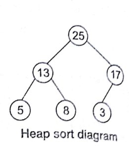
Height of node = Height of edges on a longest simple path from the node down to a leaf
Height of heap = Height of root
= (log n)
e.g., We represent heaps in level order, going from left to right. The array corresponding to the heap at the right side is [25, 13, 17, 5, 8, 3].
The root of the tree A[1] and given index i of a node, the indices of its parent, left child and right child can be computed.
Parent (
return fl oor (1/2)
Left (i )
re turn 2i
Right (i )
return 2i +1
Heap Property
The heap properties L used on the comparison of value of node and its parent are as given below
Max heap In a heap, or every node i, other than the root, the value of a node is less than or equal (atmost) to the value of its parent.
A[ parent (i)] ≥A [i]
Min heap In a heap, or every node i, other than the root, the value of a node is greater than or equal to the value of its parent.
A [parent (i)]≤A[i]
Maintaining the Heap Property
Max heapify is imp orta t for manipulating Max heap. It is used to maintain the max heap property
The following con ‘Nulls will be considered for maintaining the heap properly are given (Ds
- Before max hea,)ify, may be smaller than its children.
- Assume left and right subtree of i are max heaps.
- After max heapify, subtree rooted at i is a max heap.
Pseudo Code for Max Heapify
MaxHeapify (int a [ ],I, n)
{
int largest, temp;
int 1 =2*i;
int r = 2*i +1;
if (1._n &&a [1]>a[i])
{
largest =1;
}
else
largest = i;
if (r&& a [r] > a [largest])
{
largest = r;
}
if(largest!=i)
{
temp= a [largest];
a [largest] = a [i];
a [i] = temp;
}
MaxHeapify(a,,largest,n)
}
Basically, three basic operations performed on heap are given as
- Heapify, which runs in 0 (log2 n)
- Build heap, which runs in linear time 0(1).
- Heap sort, which runs in 0(n log2 n)
We have already discussed the first operation of heap sort. Next we will discuss how to build a heap.
Building a Heap
The following procedure given an unordered array, will produce a max heap Build
MaxHeap (int a [ ], int n)
int i;
for (i = (n/2); i >1; 1—}
{
Maxheapify (a,.i,n)
}
}
Heap Sort Algorithm
The heap sort algorithm combines the best of both merge and insertion sort. Like merge sort, the worst case time of heap sort is 0(n log2 n) and like insertion sort, heap sort is in-place sort.
Pseudo code for heap sort procedure
Heapsort (int a ], int n)
{
int i, temp;
BuildMaxHeap (a, n);
for (i =n; i >=2; ——)
{
temp= a[1];
a[1] =a [i];
a [i] = temp;
heapsize [a] = heapsize [a] —1;
}
Heapify (a, 1);
}
Analysis of Heap Sort
The total time for heap sort is 0 (n log n) in all three cases (i.e., best case, average case and worst case)
Sorting in Design and Analysis of Algorithm Study Notes with Example
Follow Us on Social Platforms to get Updated : twiter, facebook, Google Plus
Learn Sorting in Handbook Series: Click here